Web Scraping and Text Mining Lyrics
Introduction
‘Web Scraping and Text Mining Lyrics’ was an R workshop created and presented by myself and Daniel De Bortoli at both the EARL (2021) and LondonR (2022) conferences. In this blog post, we give a high level summary of the techniques used, without diving too much into the code. If you just want the code, or indeed want to follow along, feel free to take a look at the public repository. I hope this is an enjoyable read!
In the project, we used a combination of web scraping, text mining algorithms, and machine learning. Examples include sentiment analysis, topic modelling, and creating NLP features such as TFIDF and word embeddings.
Process
The process can be summarised in 3 steps:
Find track names for which we want lyrics.
Scrape the lyrics from lyric websites.
Perform analysis/machine learning on the lyrics.
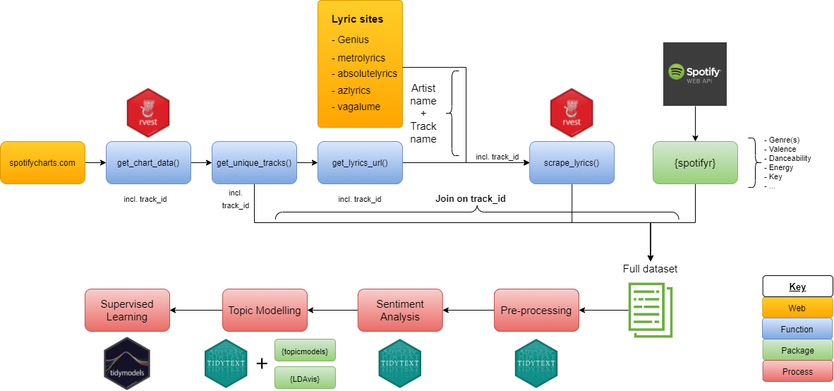
Process Diagram
Which Tracks to Use
My co-author Daniel is big into his metal music and so we thought it would be fun to use metal tracks for the project. This also set up a bit of a challenge for us as we would try later to separate 3 metal sub-genres - black metal, death metal and power metal - using only the lyrics.
In order to get tracks from these 3 sub-genres, we used the Spotify API to find playlists relating to each genre. This gave us a few thousand tracks to use.
Finding and Scraping the Lyrics
Once we had the track names and artists, we used popular lyric sites to scrape the lyrics. Often, the URL of the lyric page can be constructed in some way from the track name and artist. For example, using absolutelyrics.com, we could find lyrics for the song ‘Save Your Tears’ by The Weeknd via:
http://www.absolutelyrics.com/lyrics/view/the_weeknd/save_your_tearsDifferent lyric sites required a different URL construction, however after a little bit of cleaning (removing brackets, featured artists etc.) this was relatively straight forward. We looped through each of the sites with a tryCatch, allowing us to try lyric sites one after another, until we (hopefully) got a match on the site.
Once we had a working URL for a lyric site, we needed to actually scrape the lyrics. We looked into the HTML structure of each of the sites and used the package {rvest} to target the lyric text on the site. By looking for the right HTML tags, and using the correct CSS selector, this can be reduced to just a few lines of code. If you’re new to web scraping, check out the Selector Gadget Chrome extension, to easily find the CSS selector for the part of the website you’re trying to target.
Now that we have the lyrics for each track as a string, we can move on to the text analysis and supervised machine learning, where in the latter we will predict the metal sub-genre exclusively from the lyrics.
Text Analysis
Pre-processing
To get our lyrics ready for analysis, we need to tokenise them. This means converting the single string of lyrics that we have for each track into tokens. Tokens are simply a single unit of text, and in most cases (including our case) tokenisation just means splitting a string of lyrics into their individual words. For example, "here we go" would become "here" "we" "go". We tokenised with tidytext::unnest_tokens().
Now, when you work with text data, there’s a lot of noise. One such example are stopwords. These are words, generally used to ensure grammar, that have no significant meaning in the text, for example ‘and’, ‘to’, ‘at’, ‘by’, to name a few. Lyrics are no exception to this, and one of the first steps in our pre-processing was to remove all the stopwords. There are freely available libraries of stopwords, which we can anti_join() with our lyrics, to remove them. One such example is the dataframe built into {tidytext} - tidytext::stop_words. Below are two plots of the most common words in our lyrics, before and after removing stopwords. Don’t forget these are metal lyrics….
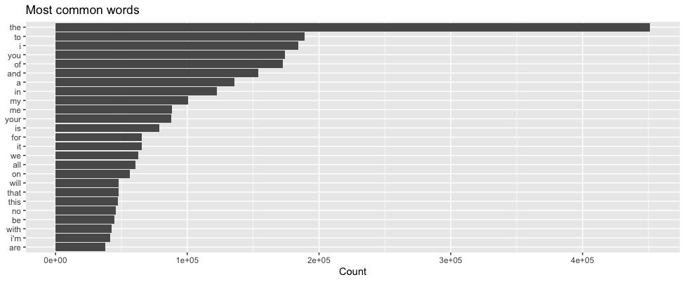
Before removing stopwords
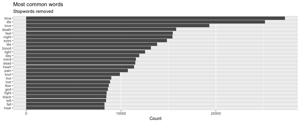
After removing stopwords
Next up is to stem our words. The concept of stemming is that words like “love”, “loving” and “loves” all have pretty much the same meaning, and for a computer to see them as totally distinct would be a mistake. Instead, we want to group these words together, by reducing them to their stem, in this case “love”.This can easily be done by applying a word-stemming algorithm, which takes a word and returns its stem. There are many different algorithms available but for 99% of words they’ll all do the same thing.
In summary, we:
Tokenised - splitting lyrics to their individual words.
Removed stopwords - words that add no analytical value e.g. prepositions.
Stemmed - reduced words to their stem, so that words deriving from the same word can be grouped.
Sentiment Analysis
Sentiment analysis is where we attempt to find the the overall sentiment of a ‘document’ (in our case a song), from the text of the document. A classic use-case is analysing online reviews, to see how positive or negative they might have been about a product. In our case, however, we look for the sentiment of the lyrics in the 3 metal genres (death, black and power metal).
Again, the {tidytext} package has multiple sentiment libraries, where words are mapped to a sentiment. Some of these libraries e.g. “afinn” return the sentiment as a score from –5 to 5. Others such as “nrc” return one of 10 worded sentiments e.g. “anger” or “surprise”.
We can analyse the sentiment of each of our tracks by joining our lyrics dataframe onto these sentiment library dataframes. Remember that after tokenising, each row in our dataframe is a word, so this is a simple left_join(). We then used the “afinn” library to get a -5 to 5 sentiment value for each word in the song lyrics, and took the average for each song. We then showed the songs for each of the 3 genres with the highest and lowest average sentiment. Once again…a reminder that these are heavy metal tracks, and so there are some explicit track names. Sorry about that…
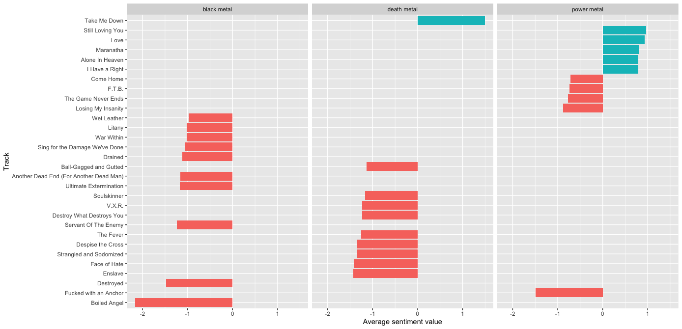
Power metal clearly stands out, with over 80% of the most positive lyrics. Black and death metal are harder to distinguish between, apart from ‘Take Me Down’ by Paradise Lost, which seems to be an anomaly. Looking at the lyrics, it’s clear how the sentiment analysis has gone wrong for this track, specifically the repetition of the word “love”, and the fact that there just aren’t many lyrics:
“You aren’t what I love, You aren’t what I need, You aren’t what I love, You aren’t what I need, What I need, No, don’t let them take me down there, Don’t let them take me down there, Don’t let them take me down there, Don’t let them take me down, You aren’t what I love, You aren’t what I see, You hate from above, You become what I need, What I need.”
Topic Modelling
Next we tried some topic modelling on the lyrics. Specifically LDA (latent dirichlet allocation), which is one of the most popular topic modelling techniques. In LDA, you give a number of topics (k) to an algorithm, along with your ‘documents’ (songs) and their lyrics. The algorithm will then try to group them into k topics. It does this by assigning songs to different topics, and then seeing which words are common amongst songs in the same topic, however not common amongst songs in a different topics. Starting with a random allocation of songs to topics, it updates:
- The probability of a word occurring in a topic, given the songs associated with that topic.
- The probability of a certain song being in a topic, given the words in that song.
This eventually converges and we have k topics along with probabilities for each word being associated with that topic. In our analysis, we chose k=3 and hoped that we’d naturally end up seeing a topic as a genre, i.e. one for black, death and power metal. After running the algorithm, we plotted the top words associated with each topic, shown below:
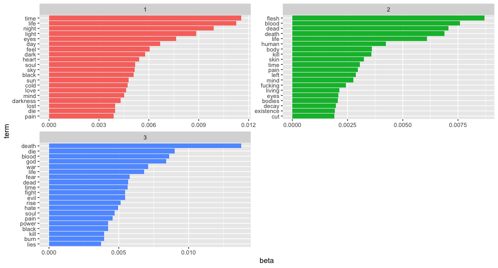
And it basically worked! We can see that topic 3 is quite clearly power metal - lots of mythical/epic/fight type themes. Topic 2 is also clearly death metal, with a lot of gore going on in the top words. Black metal also fits topic 1 quite well with lots of mentions darkness, night, light, sun etc.. We can also look at which genres contains the highest average song probability for association with each topic.
## # A tibble: 3 × 4
##   genre          p1    p2    p3
##   <chr>       <dbl> <dbl> <dbl>
## 1 black metal  0.32  0.56  0.12
## 2 death metal  0.23  0.43  0.34
## 3 power metal  0.16  0     0.83
Looking down the columns, we see that genre that most lines up with each of our topics is exactly the genre we expected. It’s also interesting to note that despite topic 1 being most associated with black metal, both black metal and death metal are more likely to fall into topic 2 than any other topic. This may seem slightly counter-intuitive, but that’s the way LDA models work, in that multiple topics will occur in a single document. We therefore need to look at how often topics occur in each document in relation to how often they occur in the rest of the documents to get a sense for what topic ‘stands out’ from that document.
Supervised Machine Learning
Next we tried to formally predict the genre of each song, purely based on their lyrics. To do this, you have to create features for your ML model. There are a few ways of doing this, and we tried two of the most popular, TFIDF and word embeddings.
TF-IDF
TFIDF stands for text frequency - inverse document frequency. Essentially, it’s a measure of how common a word is in a document, compared with how common it is in the rest of the documents in our dataset (our corpus). It’s actually a very simple thing to measure, although having said that there are a few different ways this is done.
The most simple way